Try the Free Math Solver or Scroll down to Tutorials!

Enter expression, e.g. (x^2-y^2)/(x-y)

Enter expression, e.g. x^2+5x+6

Enter expression, e.g. (x+1)^3

Enter a set of expressions, e.g. ab^2,a^2b

Enter equation to solve, e.g. 2x+3=4

Enter equation to graph, e.g. y=3x^2-1

Depdendent Variable

Number of equations to solve:

Equ. #1:

Equ. #2:

Equ. #3:

Equ. #4:

Equ. #5:

Equ. #6:

Equ. #7:

Equ. #8:

Equ. #9:

Solve for:

Enter inequality to solve, e.g. 2x+3>4

Enter inequality to graph, e.g. y<3x^2-1

Dependent Variable

Number of inequalities to solve:

Ineq. #1:

Ineq. #2:

Ineq. #3:

Ineq. #4:

Ineq. #5:

Ineq. #6:

Ineq. #7:

Ineq. #8:

Ineq. #9:

Solve for:

Math solver on your site

Please use this form if you would like
to have this math solver on your website,
free of charge.

Name:

Email:

Your Website:

Msg:

Another Worksheet for Logistic Growth

Summary and expansion of discussion in the book: In a logistic growth model, calculate mL:
Then one of the following cases must apply:

• If mL ≤ 1 the population will die off for any initial population size between 0 and L:

• If 1 < mL ≤ 3 the population will level off eventually, for any initial population size
between 0 and L. The steady population size will be L - 1/m.

• If 3 < mL ≤ 4, the population may not level off. However, you can be sure that the model
will always produce population values that stay between 0 and L; provided the initial
population size is between 0 and L:

• If mL > 4; the model may eventually produce negative values for population size. This is
invalid and shows that the model is unreliable for future predictions.

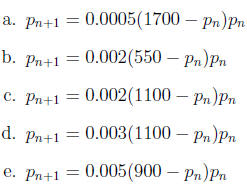
1. In the first logistic growth worksheet, you were supposed to develop logistic growth models for
growing mold in a laboratory under a variety of conditions. The difference equations that you
should have found are shown below. For each one, use the results of the logistic growth chapter
to decide if the population eventually dies out, levels off, remains valid without leveling off, or
eventually leads to negative (and so invalid) predicted population sizes.

2. For model c above, investigate the effect of harvesting various amounts from the model. For
example, if you harvest 100 members of the population from each cycle, the difference equation
will become

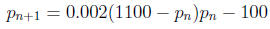
Describe what will happen to this population over the long term. Does it matter what the
starting population is?

3. Repeat the preceding problem using a harvest of 160, then of 200.

Summary and expansion of discussion of harvesting: In a logistic growth model with harvesting,
the difference equation has the following form:

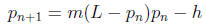
where h is the amount harvested for each cycle. The long term behavior of this model is determined
by the roots of the equation

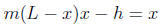
which are the fixed points of the model. To find them, express the equation in the form

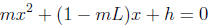
and use the quadratic formula. Generally there are two roots, which can be referred to as LFP
(for lower fixed point) and HFP (for higher fixed point). If these are both between 0 and L,
then the following conclusions hold:

• If the initial population is any number between LFP and L - LFP, the model will eventually
level off and remain at a size equal to HFP.

• If the initial population is between 0 and LFP the model will decrease and eventually
become negative.

• If the initial population is between L-LFP and L the model will decrease and eventually
become negative.

• If there are no roots to the equation above, the model will decrease and eventually become
negative no matter what the starting population size is.

For each of the problems with harvesting on the preceding page, find LFP, HFP, and L-HFP.
Use the summary above to analyze the future behavior of the model, and compare with the results
you found for problems 2 and 3 earlier.

Home